EverLight: Indoor-Outdoor Editable HDR Lighting Estimation — Supplementary Material — ICCV 2023
This document provides additional results and analysis for our proposed method in the main paper. We start with showcasing the power of our approach for editing by conducting an experiment on changing the position of input lighting parameters and visualizing the corresponding output. Next, we show different editing results for various indoor and outdoor input images. Then, we provide further results for outdoor and indoor scenarios. We conclude this document by providing more implementation details on our method.
Table of Contents
- Moving lighting parameters (extends fig. 6)
- Editing (extends fig. 6)
- Outdoor Results (extends fig. 5)
- Indoor Results (extends fig. 4)
- Implementation Details
1. Moving Lighting Parameters
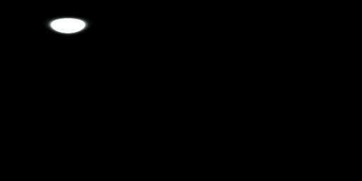
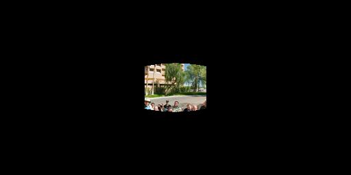
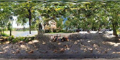
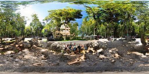
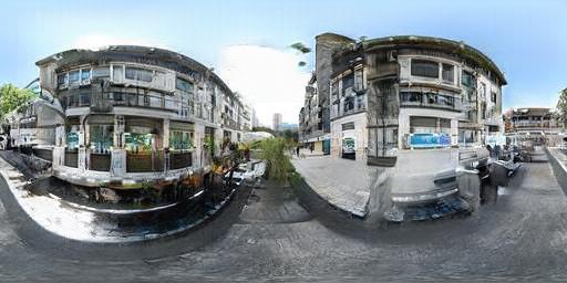
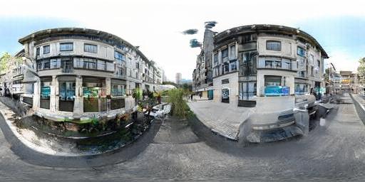
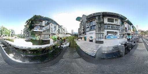
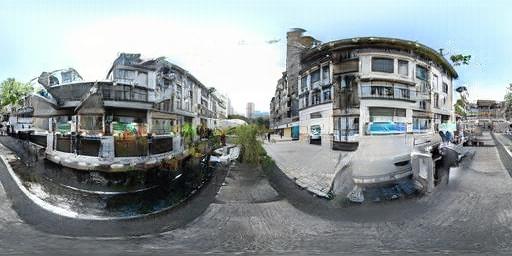
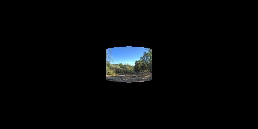
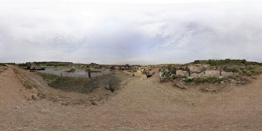
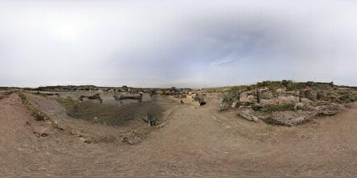
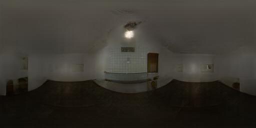
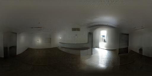
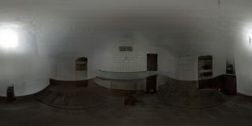
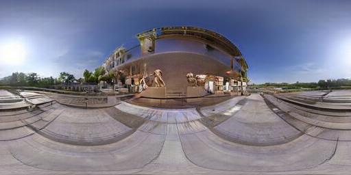
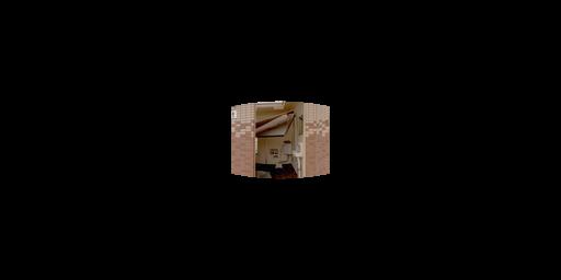
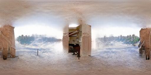
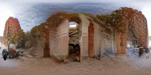
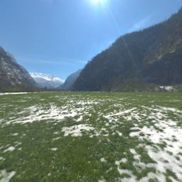
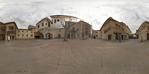
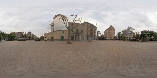
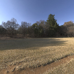
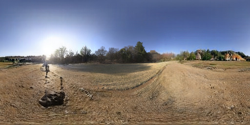
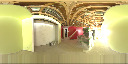
To show the performance of our method for editing, we change the position of lighting parameters smoothly, and as a result, we create a video of the output of the network.
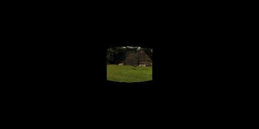
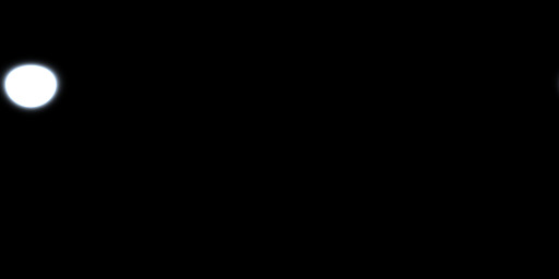
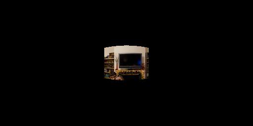
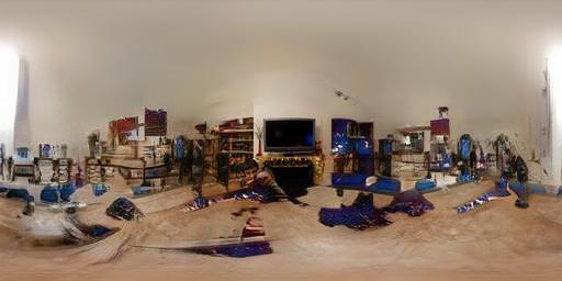
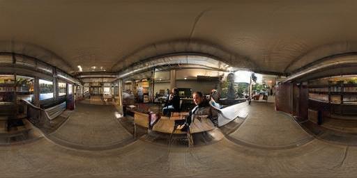
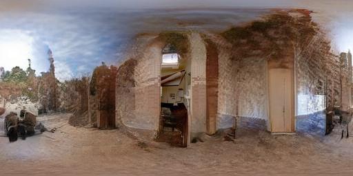
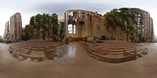
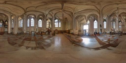
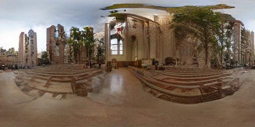
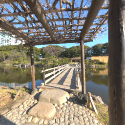
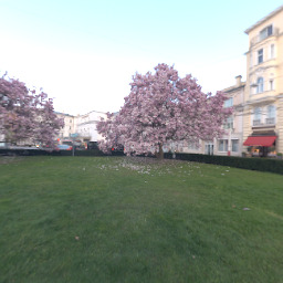
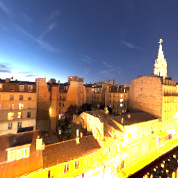
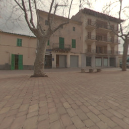
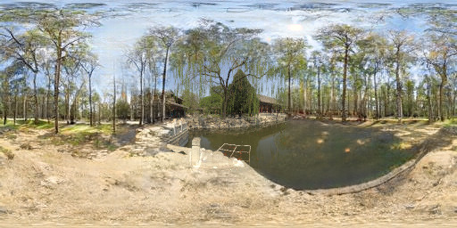
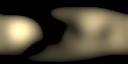
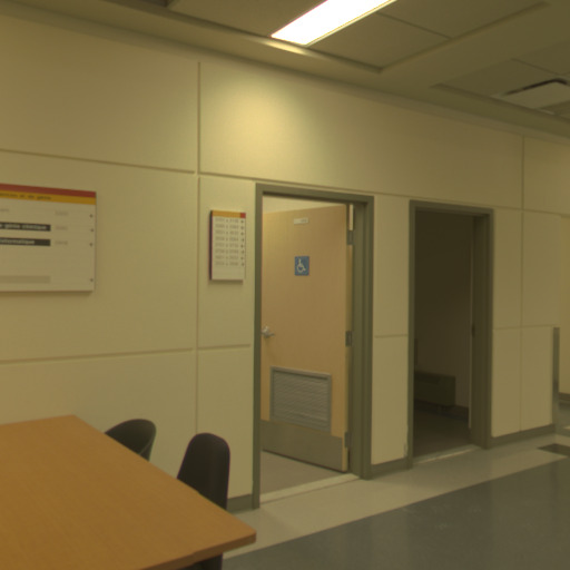
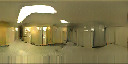
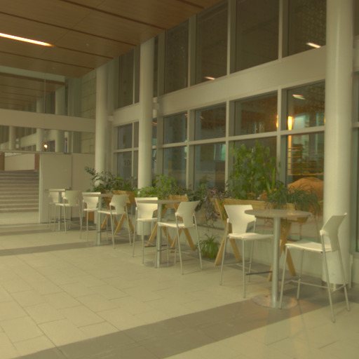
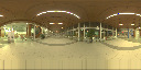
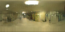
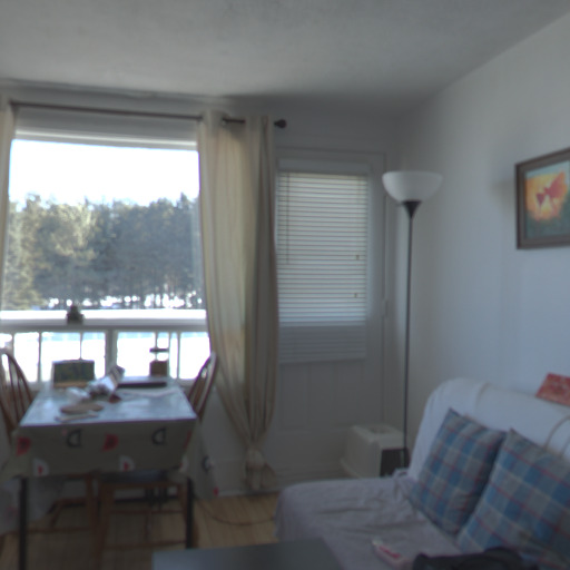
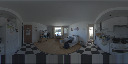
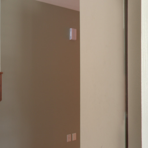
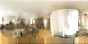
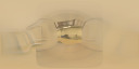
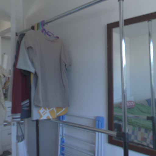
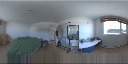
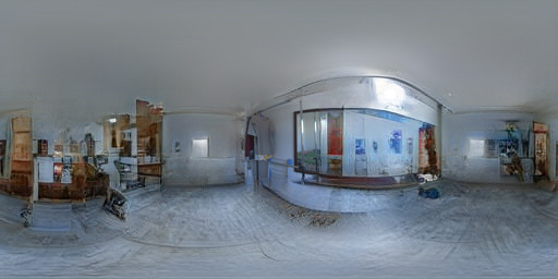
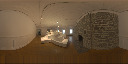
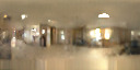
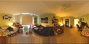
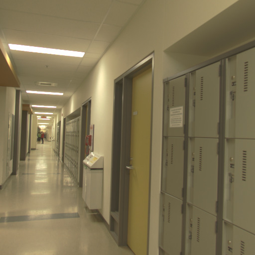
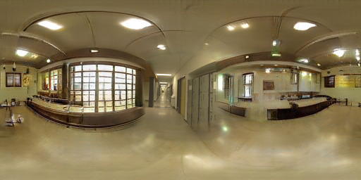
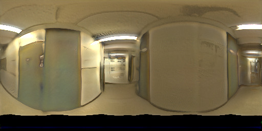
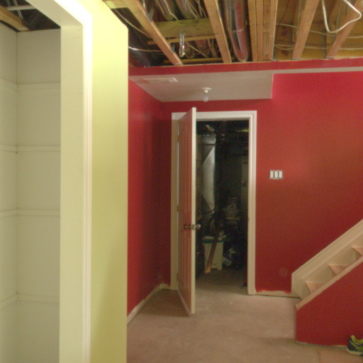
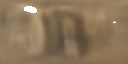
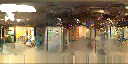
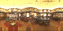
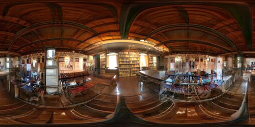
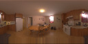
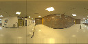
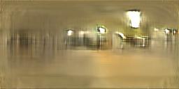
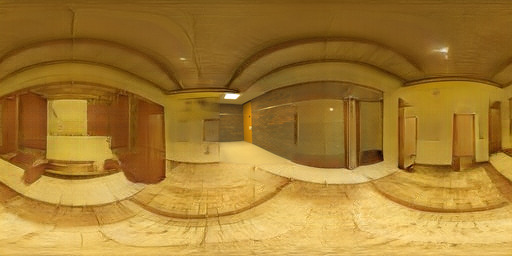
Input image
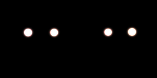
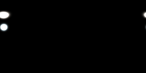
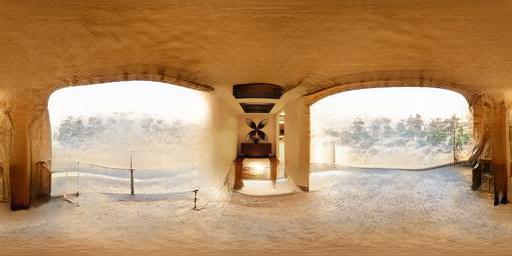
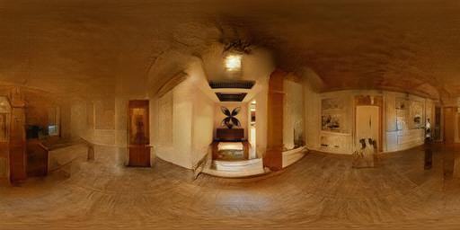
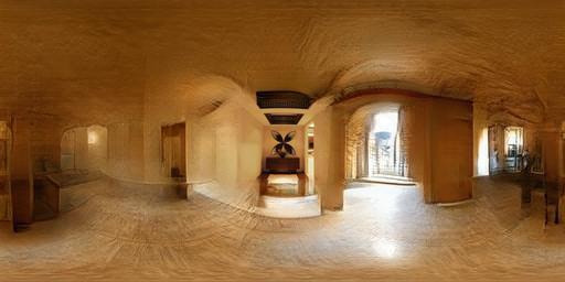
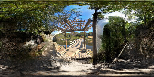
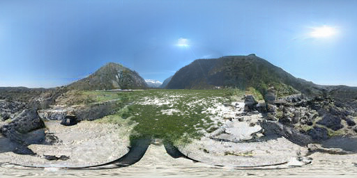
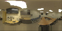
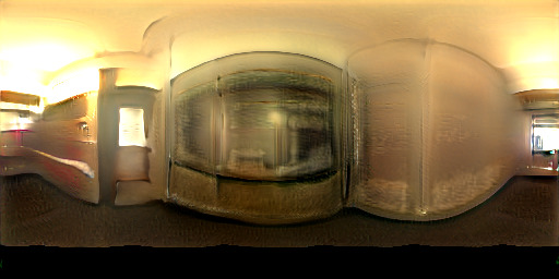
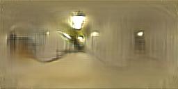
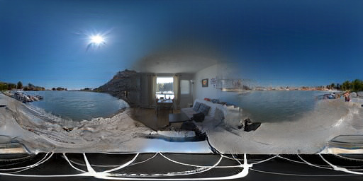
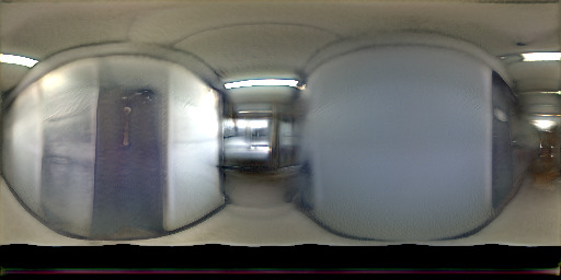
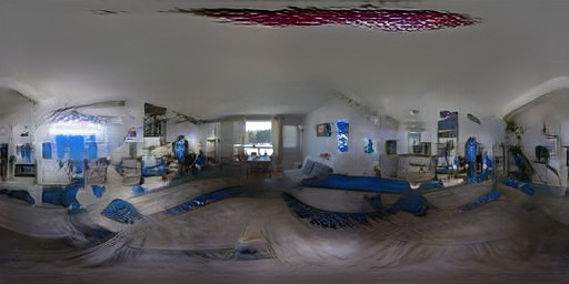
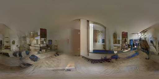
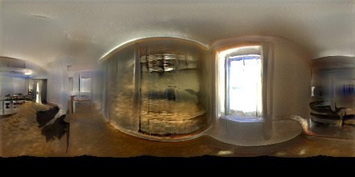
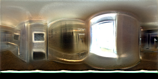
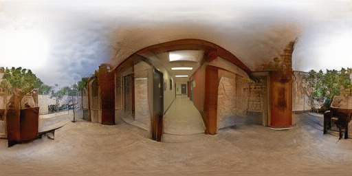
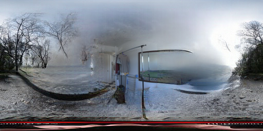
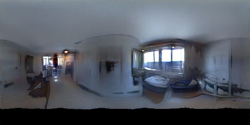
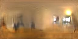
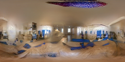
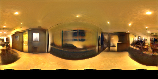
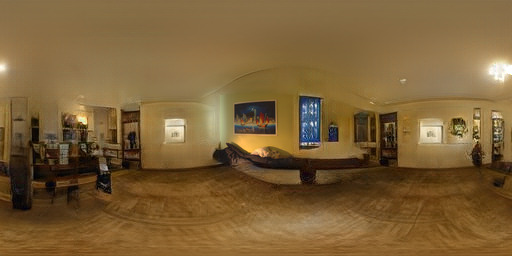
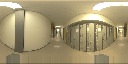
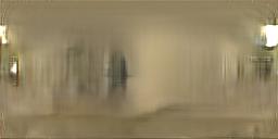
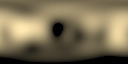
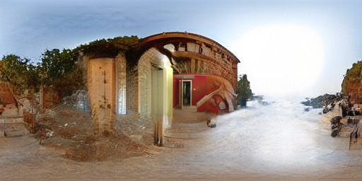
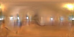
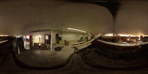
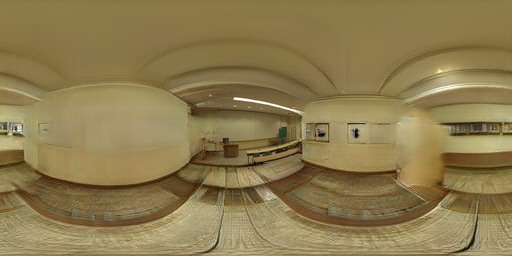
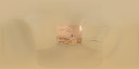
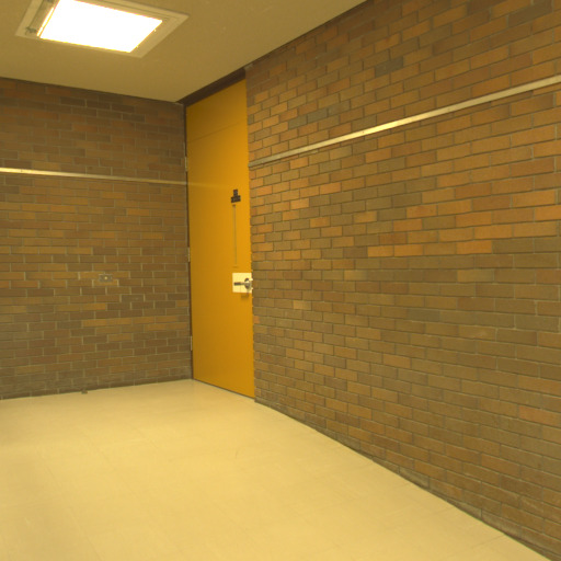
Input lighting parameters and the corresponding output
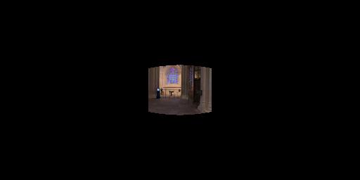
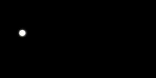
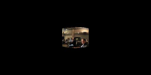
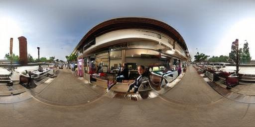
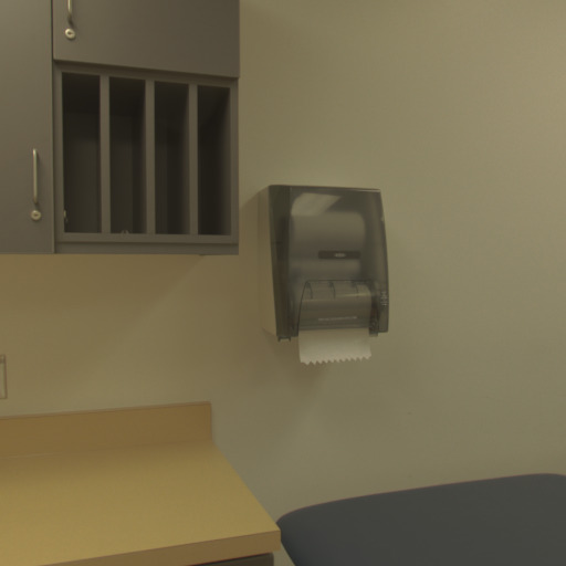
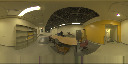
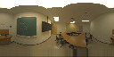
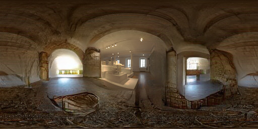
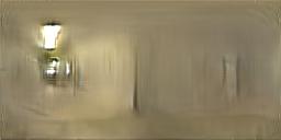
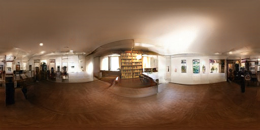
Input image
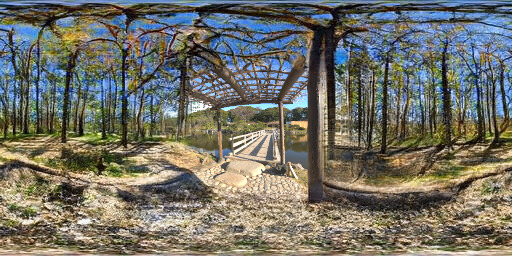
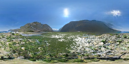
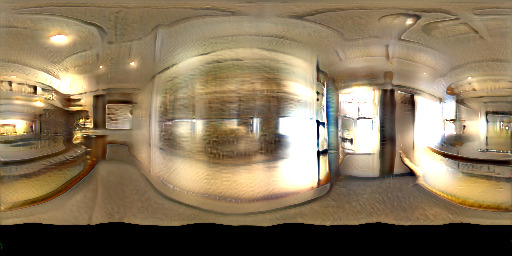
Input lighting parameters and the corresponding output
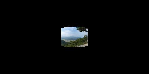
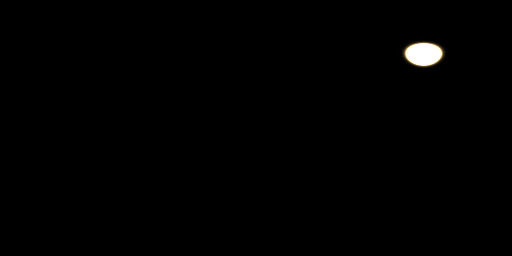
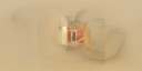
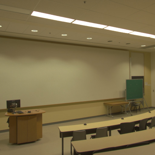
Input image
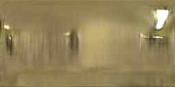
Input lighting parameters and the corresponding output
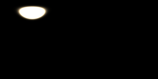
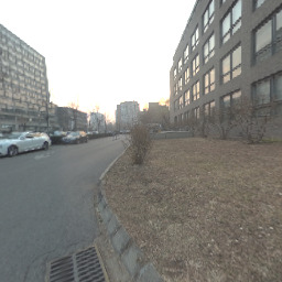
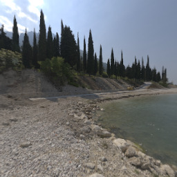
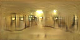
Input image
Input lighting parameters and the corresponding output

Input image
Input lighting parameters and the corresponding output
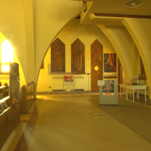
2. Editing results
Here are more results of our method for different lighting user inputs as an extension to figure 6. Please consult section 5.3 of the main paper for more information. First we show results for outdoor cases.


Our method works well for both outdoor and indoor scenarios. Here are more results of our method for different lighting user inputs for indoor cases.


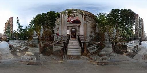


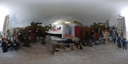


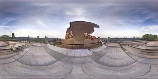
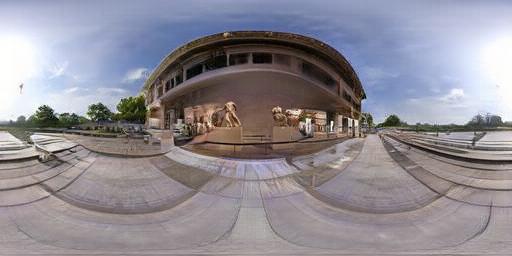


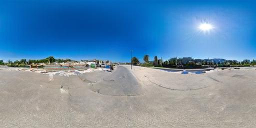
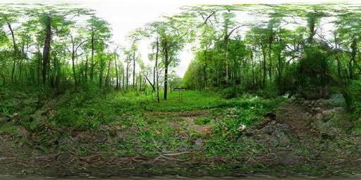
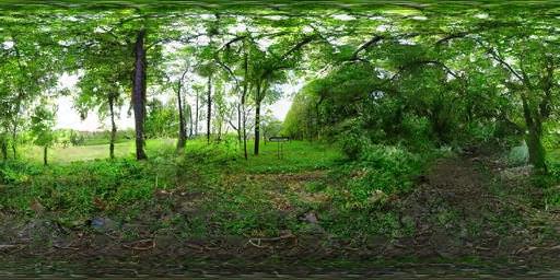
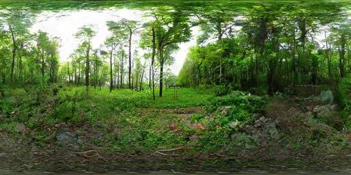
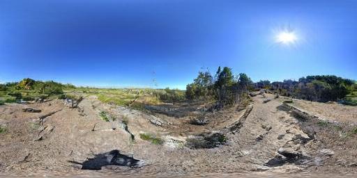
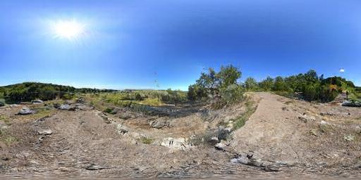
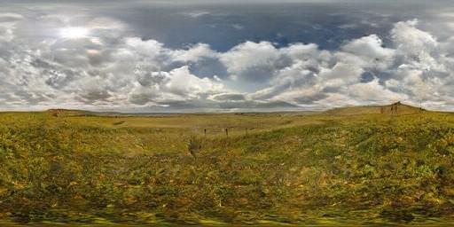
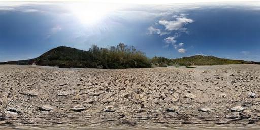
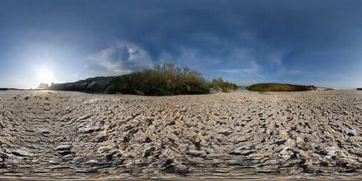
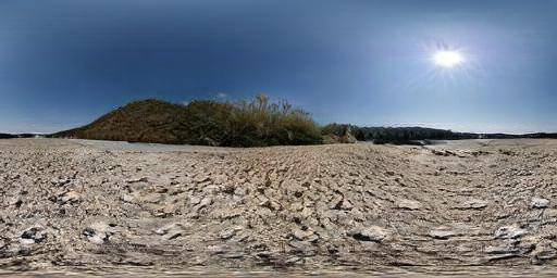
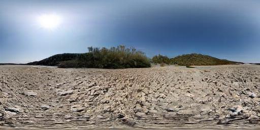
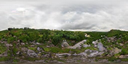
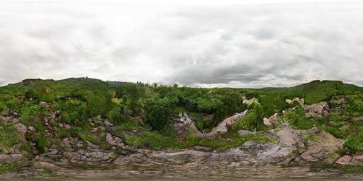
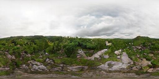
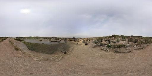
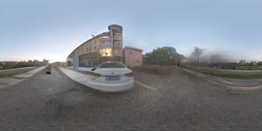
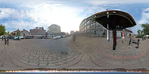
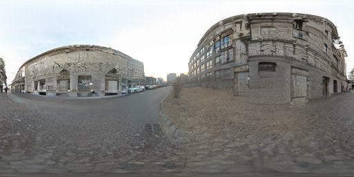
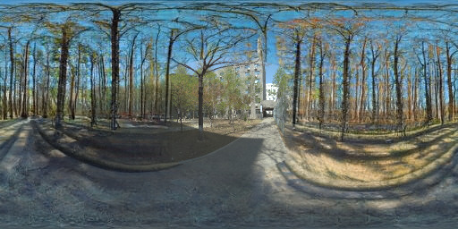
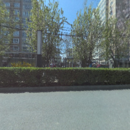
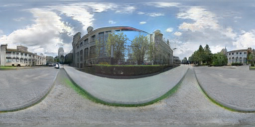
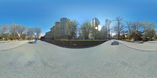
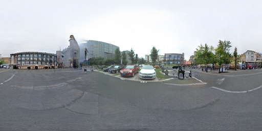
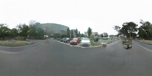
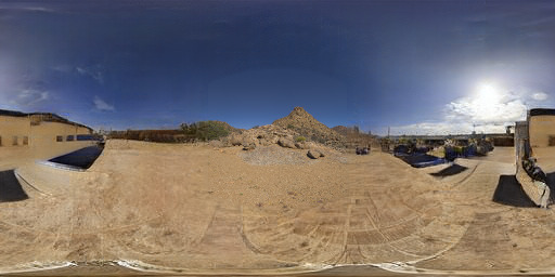
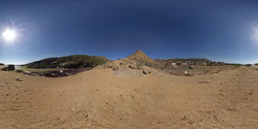
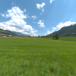
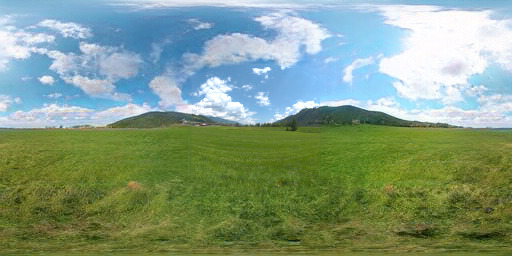
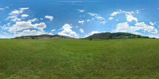
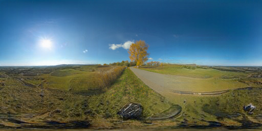
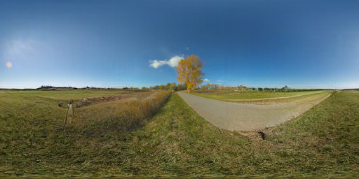
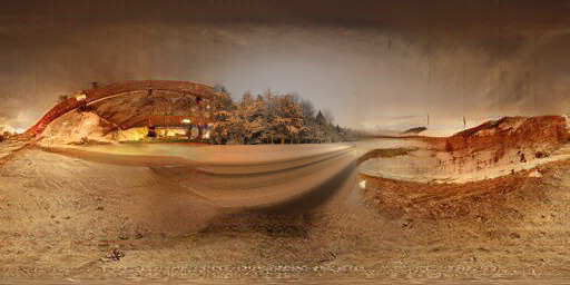
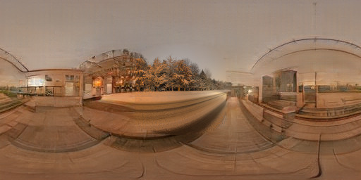
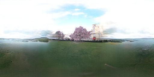
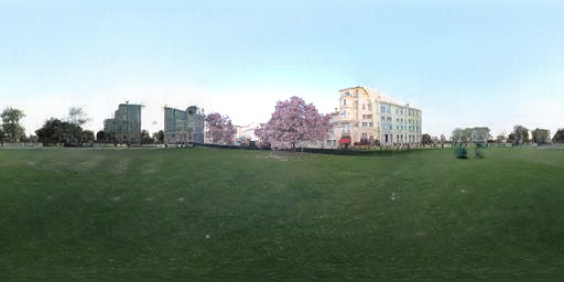
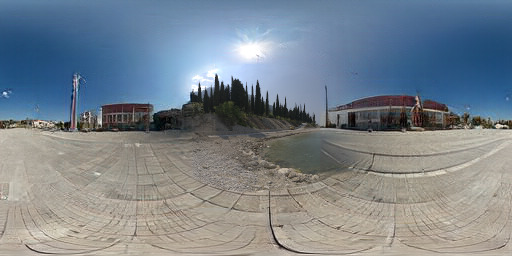
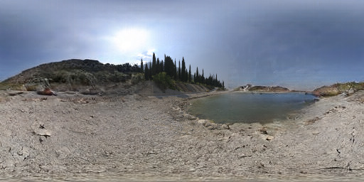
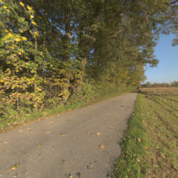
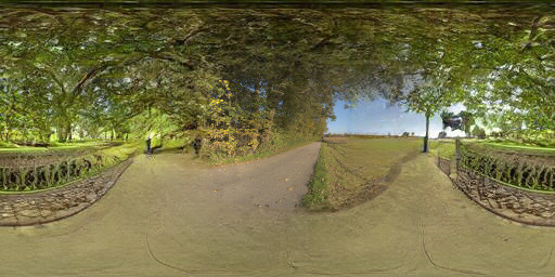
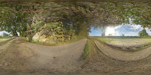
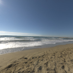
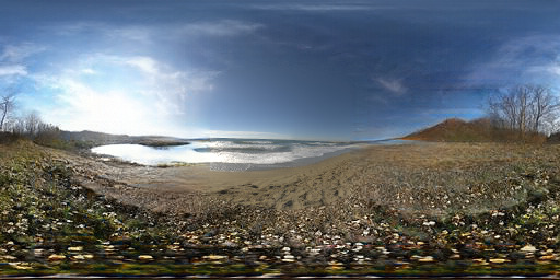
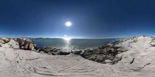
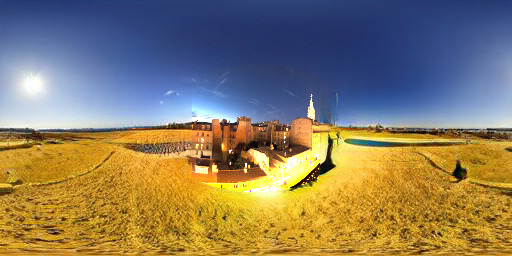
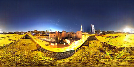
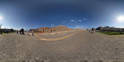
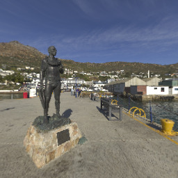
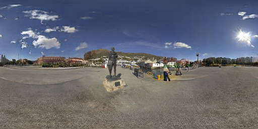
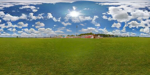
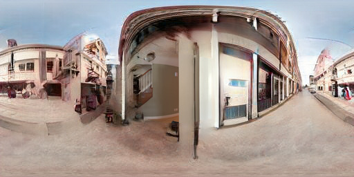
3. Outdoor Results
Here are more results of our method compared to existing methods for outdoor cases as an extension to figure 5. Please consult section 5.2 of the main paper for more information.
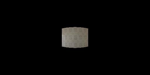
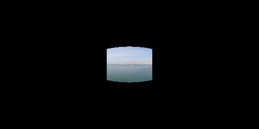
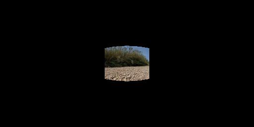
Input Crop
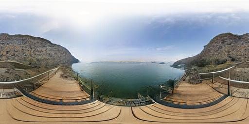
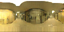
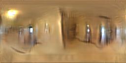
immersegan [6]
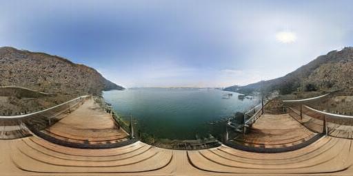
Zhang’19 [59]
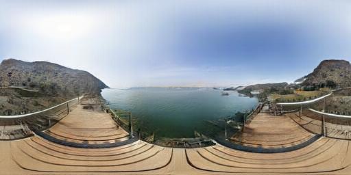
EverLight (ours)


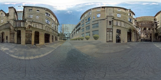

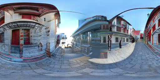

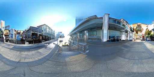


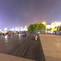
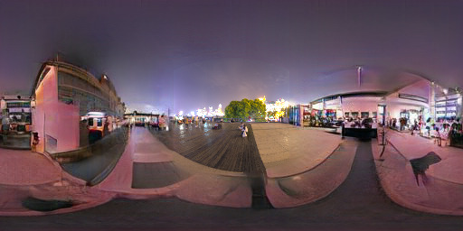


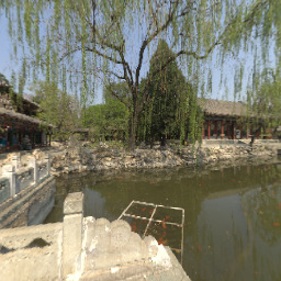
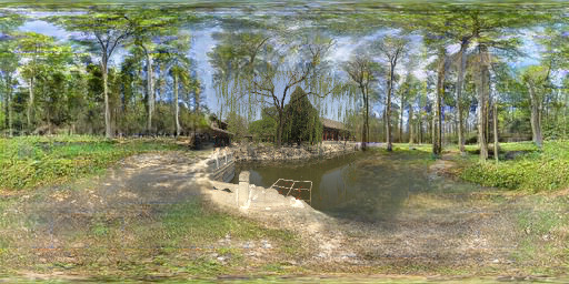

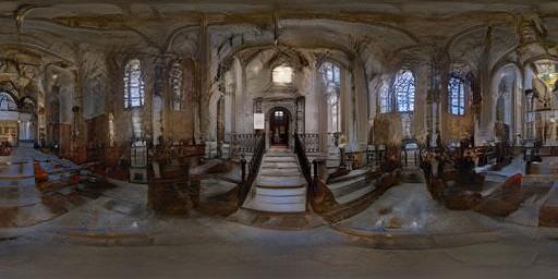
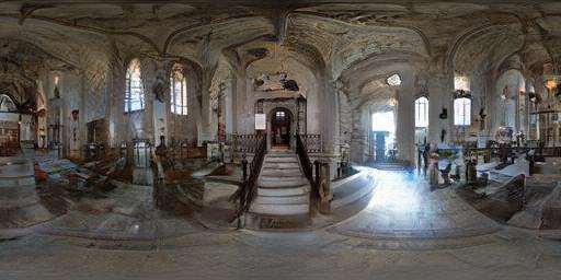
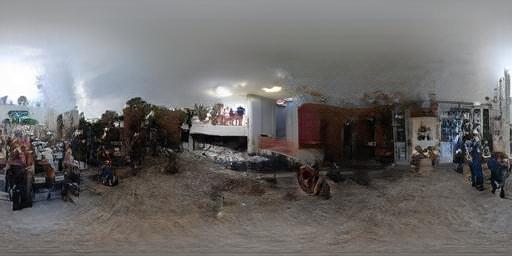
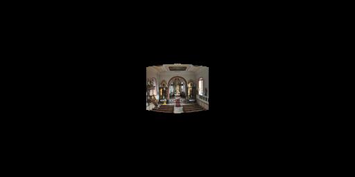
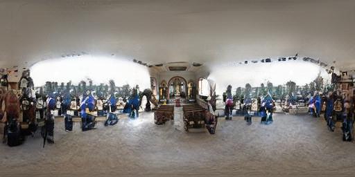
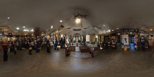
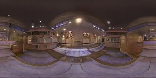
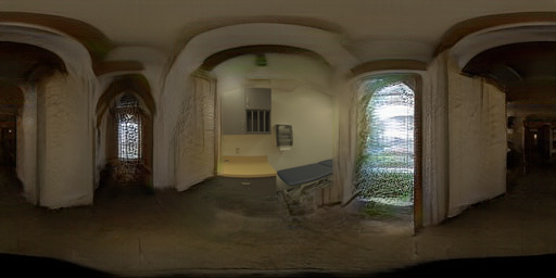
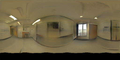
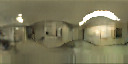
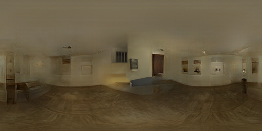
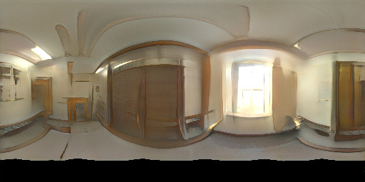
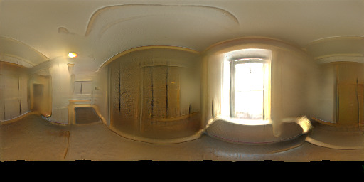
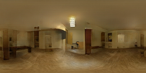
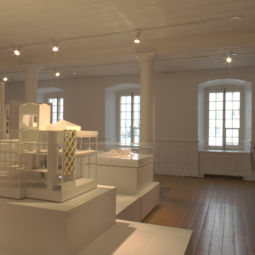
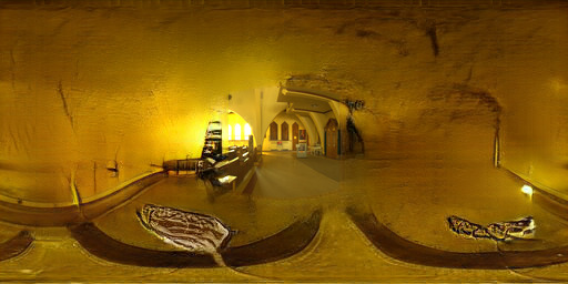
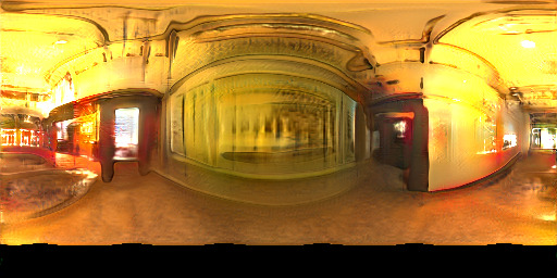
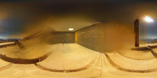
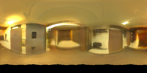
4. Indoor Results
Here are more results of our method compared to existing methods for outdoor cases as an extension to figure 4. Please consult section 5.1 of the main paper for more information.


5. Implementation Details
As described in sec. 4.3 of the main manuscript, our spherical gaussian fitting \( f_\mathrm{SG}^{-1} \) is performed using the following optimization: \[ \hat{\mathbf{p}} = \arg\min_{\mathbf{p}} \sum_{\omega \in \Omega} \lambda_1 \left\lVert f_\mathrm{SG}(\omega; \mathbf{p}) - \mathbf{E}(\omega) \right\rVert_2^2 + \ell_\mathrm{reg}( \mathbf{p} ) \; ,\] recovering the light parameters \( \hat{\mathbf{p}} \) from the environment map \( \mathbf{E}(\omega) \). Please see the main manuscript for the description of the first term. The second term \( \ell_\mathrm{reg}( \mathbf{p} ) \) is a regularizing term used to stabilize the optimization over light vector length \( \ell_\mathrm{length} \), intensity positivity \( \ell_\mathrm{neg} \), light color \( \ell_\mathrm{color} \) and bandwdith \( \ell_\mathrm{sigma} \). We sum the regularizing terms as \[ \ell_\mathrm{reg}( \mathbf{p} ) = \lambda_2 \ell_\mathrm{length} + \lambda_3 \ell_\mathrm{neg} + \lambda_4 \ell_\mathrm{color} + \lambda_5 \ell_\mathrm{\sigma} \; . \] In the following, we describe each individual term.
The vector length loss \( \ell_\mathrm{length} \) is used since the representation for the light position used during the optimization is \( \xi \in \mathcal{R}^3 \), effectively optimizing over the cartesian coordinates \( \{x,y,z\} \). While this yields one additional degree of freedom over the necessary \( \mathcal{S}^2 \) space required to represent all 3D rotations, we found this representation to be more stable due to the lack of wraparound. As such, we need to constrain the cartesian coordinates to be close to unit length during the optimization, which we do using \[ \ell_\mathrm{length} = \sum_{k=1}^K \left\vert 1 - \left\Vert \xi_{k_{\{x,y,z\}}} \right\Vert \: \right\vert \; ,\] where \( \left\Vert \cdot \right\Vert \) is the vector length, and \( \left\vert \cdot \right\vert \) the absolute value. This loss is summed over all lights \( K \).
We enforce the light color to be non-negative using \[ \ell_\mathrm{neg} = \sum_{k=1}^K \left\vert \max(\mathbf{c_k}, 0) \right\vert \; , \] ensuring values of light intensity \( \mathbf{c_k} \) below 0 are penalized. Similarly, we regularize the light color towards gray using \[ \ell_\mathrm{color} = \sum_{k=1}^K \left\vert \delta_{\left\vert \mathbf{c_k} \right\vert,1\!\times\!10^{-3}} \cdot \sigma_\mathbf{c_k} \right\vert \; , \] where \( \sigma_\mathbf{c_k} \) is the standard deviation of the rgb values of light \(k\), and \( \delta_{\left\vert \mathbf{c_k} \right\vert,1\!\times\!10^{-3}} \) is the Kronecker delta function taking the value 1 when the intensity of light \( \mathbf{c_k} \) is over \( 1\!\times\!10^{-3} \) and 0 otherwise.
Finally, we found that leaving the light bandwidth—or effective size—\( \sigma_k \) unconstrained during the optimization would typically result in very large lights, potentially yielding almost uniform lights on the sphere. We hypothesize the optimization tries to approximate ambient light with very large \( \sigma_k \) values. To circumvent this, we use the following loss: \[ \ell_\mathrm{\sigma} = \sum_{k=1}^K \max \left(\sigma_k, \; \sqrt{\frac{0.05}{4\pi}} \right) \;. \] In our implementation, \( \lambda_2 = 0.1 , \lambda_3 = 10 , \lambda_4 = 1\!\times\!10^{-2} , \lambda_5 = 0.8 \).