SpotLight: Shadow-Guided Object Relighting via Diffusion — Supplementary Material
We present additional results complementing the main paper. In particular, we show interactive relighting results,
using pre-computed images generated by our method and baselines.
Hover your mouse over the images to see animated relighting results!
Table of Contents
- Technical details on the shadow blending (extends sec. 4.2)
- RGB-X backbone (extends sec. 5.2)
- Lighting-conditioned methods parametrization (extends sec. 5.3.2)
- Additional quantitative results (extends sec. 5.4, tab. 1 and tab. 2)
- Additional qualitative results (extends sec. 5.4, fig. 3) (Interactive)
- User studies (extends sec. 5.5)
- Parameters control (extends sec. 5.6) (Interactive)
- Light source radius (extends sec. 5.6) (Interactive)
- Outdoor scenes (extends sec. 6)
- Diverse objects (extends sec. 6)
- Multiple lights (extends sec. 6) (Interactive)
- Full image relighting (extends sec. 6) (Interactive)
1. Technical details on the shadow blending
Here we further detail how we obtain the latent shadow mask \(\mathbf{m}_{\text{shw},\downarrow}\) from the full resolution guiding shadow \(\mathbf{m}_{\text{shw}}\). We first downsample the shadow \(\mathbf{m}_{\text{shw}}\) by simple bilinear interpolation. We then binarize the downsampled shadow using a threshold of 0.05 (to include the softer parts of the shadow in the mask). We dilate the mask using a \(3\times 3\) kernel to include the details at the edge, and further multiply by two the mask value at the edge. Finally, we remove from the shadow mask its intersection with the downsampled object mask, to avoid the shadow from leaking in the object shading, in the latent space.
2. RGB-X backbone
We employ the checkpoint of their X->RGB model finetuned for inpainting rectangular masks, and mask out the bounding box including both the object and shadow region. To estimate intrinsic properties of test images (normals, metallic, roughness, and albedo), we use the RGB->X model. We observe that results are generally overly bright, likely due to a domain gap between the training and evaluation images. To address this, we re-expose the background by a factor of 2 before feeding it to the network, then divide the output by 2, in linear space. We apply the same background preservation strategy as in ZeroComp.
We show quantitative and qualitative results of the RGB-X backbone in sections 4 and 5 of this supplementary material.
3. Lighting-conditioned methods parametrization
Both DiLightNet and Neural Gaffer require an environment map for lighting. We construct such an environment map with radiance \(L_{\text{env}}\) along direction \(\omega\) defined as the sum of a spherical gaussian and a constant term \begin{equation} L_{\text{env}}(\omega) = \mathbf{c}_\text{light} e^{\lambda (\omega \cdot \mathbf{v} - 1)} + \mathbf{c}_\text{amb} \,, \end{equation} where \(\mathbf{c}_\text{light}\) and \(\mathbf{c}_\text{amb}\) are the RGB colors of the light and ambient terms resp., \(\mathbf{v}\) is the dominant light source direction, and \(\lambda\) is the bandwidth. \(\mathbf{c}_\text{amb}\) is obtained by computing the average color over the background image. Panoramas from the Laval Indoor HDR dataset (excluding those in our test set) are used to estimate a single average intensity of the dominant light source, \(k\), which is set to the ratio of the integral of the brightest pixels in the panoramas, divided by the integral over all pixels. We further divide this integral by 2 to consider a single hemisphere and avoid overly bright dominant light sources. The light color is defined by \(\mathbf{c}_\text{light} = k \mathbf{c}_\text{amb}'\), where \(\mathbf{c}_\text{amb}'\) is the normalized ambient color \(\mathbf{c}_\text{amb}\). We found that the bandwidth parameter \(\lambda\) did not advantage any specific method and therefore fixed it to \(\lambda = 300\), which we typically observe for an indoor light.
4. Additional quantitative results
We extend the quantitative results from tab. 1. First, we compute metrics separately for the foreground (evaluating the fidelity of the object's shading compared to the ground truth) and the background (evaluating the fidelity of the background shadows compared to the ground truth). Then, we include additional results, including SpotLight applied to the RGB-X backbone.
| Method | Full image | Foreground only | Background only | |||||||
|---|---|---|---|---|---|---|---|---|---|---|
| PSNR | SSIM | RMSE | MAE | LPIPS | RMSE | MAE | SI-RMSE | RMSE | MAE | |
| DiLightNet | 24.67 | 0.948 | 0.064 | 0.022 | 0.042 | 0.207 | 0.192 | 0.055 | 0.03 | 0.009 |
| Neural Gaffer | 28.44 | 0.963 | 0.042 | 0.015 | 0.038 | 0.102 | 0.088 | 0.049 | 0.03 | 0.009 |
| IC-Light | 26.87 | 0.959 | 0.054 | 0.019 | 0.04 | 0.153 | 0.13 | 0.062 | 0.03 | 0.009 |
| ZeroComp+SDEdit | 26.0 | 0.938 | 0.053 | 0.025 | 0.079 | 0.079 | 0.064 | 0.048 | 0.048 | 0.022 |
| SpotLight (no guidance) | 31.69 | 0.976 | 0.029 | 0.011 | 0.029 | 0.086 | 0.073 | 0.046 | 0.017 | 0.006 |
| SpotLight (with guidance, ours) | 30.68 | 0.974 | 0.033 | 0.012 | 0.03 | 0.1 | 0.085 | 0.05 | 0.018 | 0.006 |
| SpotLight (RGB-X backbone) | 26.56 | 0.955 | 0.051 | 0.018 | 0.042 | 0.176 | 0.155 | 0.06 | 0.02 | 0.007 |
We also extend the results from tab. 2, showing the results of the full image, foreground only, and background only for the latent mask weight β and guidance scale γ in the following two tables. We observe that some changes in parameters, like using no blending (β=0), or using no guidance (γ=1) may provide better quantitative results. However, we observe in our qualitative evaluation and user studies that these changes diminish the level of light control over the object. Our selected parameter combination provides good quantitative performance and adequate lighting control.
| Method | Full image | Foreground only | Background only | |||||||
|---|---|---|---|---|---|---|---|---|---|---|
| PSNR | SSIM | RMSE | MAE | LPIPS | RMSE | MAE | SI-RMSE | RMSE | MAE | |
| SpotLight (γ=1, no guidance) | 31.69 | 0.976 | 0.029 | 0.011 | 0.029 | 0.086 | 0.073 | 0.046 | 0.017 | 0.006 | SpotLight (γ=3, with guidance, ours) | 30.68 | 0.974 | 0.033 | 0.012 | 0.03 | 0.1 | 0.085 | 0.05 | 0.018 | 0.006 |
| SpotLight (γ=7) | 28.68 | 0.966 | 0.043 | 0.015 | 0.036 | 0.138 | 0.116 | 0.062 | 0.019 | 0.006 |
| Method | Full image | Foreground only | Background only | |||||||
|---|---|---|---|---|---|---|---|---|---|---|
| PSNR | SSIM | RMSE | MAE | LPIPS | RMSE | MAE | SI-RMSE | RMSE | MAE | |
| SpotLight (β=0.2) | 29.24 | 0.969 | 0.039 | 0.014 | 0.034 | 0.102 | 0.086 | 0.051 | 0.025 | 0.008 | SpotLight (β=0.05, ours) | 30.68 | 0.974 | 0.033 | 0.012 | 0.03 | 0.1 | 0.085 | 0.05 | 0.018 | 0.006 |
| SpotLight (β=0, no blending) | 30.81 | 0.974 | 0.032 | 0.012 | 0.029 | 0.098 | 0.083 | 0.05 | 0.018 | 0.006 |
5. Additional qualitative results
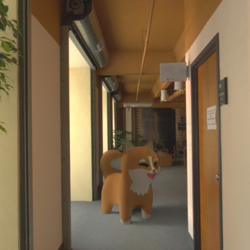
We present 20 additional randomly-selected results on the "user-controlled" dataset, extending the
qualitative results from fig. 5.
In this case, we rendered 8 light directions instead
of 5 (as used for the user study), in order to also show results where the shadow is behind the object.
Move your mouse from left to right over the images to see the light direction change.
6. User studies
6.1 Additional user studies on object shading and shadows only
In addition to the overall realism and lighting control user studies, we conducted two user studies to disentangle the shadow from the shading realism. To evaluate shading realism, the shadow needs to be fixed for all methods. To do so, for all methods, we replace the region outside the object mask by the output of SpotLight, containing a refined shadow. To evaluate shadow realism, we do the opposite. We replace the region within the object mask by the output of SpotLight, containing the shaded object. We show the results of these two user studies below.
.svg)
.svg)
On the task of refining the guiding shadow into a realistic one, SpotLight achieves higher results than both ZeroComp+SDEdit and using the guiding shadow directly. We attribute this to our shadow blending strategy, which acts as a soft constraint over the shadow generation at each denoising timestep.
6.2 Additionnal lighting control study
In addition to the lighting control user study in fig. 4b, that compares our method to the ZeroComp+SDEdit, we show here that disabling the guidance term yields a similar degradation in perceptual scores for the lighting control setting.
 vs SDEdit.svg)
 vs CFG=1.svg)
6.3 Further details
User study randomization
To use the Thurstone case V Law of comparative judgement, we need a fixed set of comparisons, shown to all observers. This set of comparison is randomly sampled and reused for all users. To limit bias, the method left/right ordering is randomized, and the order of comparisons was randomized for each observer. All user studies were conducted using different sets of observers, to avoid bias.
Observer filtering
For each study, three sentinels images were randomly placed in the questions. Incorrectly selecting one of the sentinel answers led to exclusion. In the realism user studies, the sentinels corresponded to the object set to be full white, therefore having highly unrealistic shading. For the light control user studies, the sentinels corresponded to an object where the object's lighting doesn't change as the shadow moves.
Per-study details
Here, we show the details of each user study. "Filtered observers" represents the number of observers that ended up contributing to the scores, which were selected since they didn't click the sentinels. Also note that the number of questions shown includes the three sentinel questions asked to the users.
| User study name | Original observers | Filtered observers (N) | Questions per method pairs | Total questions |
|---|---|---|---|---|
| Overall realism | 40 | 35 | 20 | 123 |
| Shadow realism | 14 | 13 | 40 | 123 |
| Shading realism | 14 | 11 | 40 | 123 |
| Lighting control (vs. ZeroComp+SDEdit) | 10 | 8 | 40 | 43 |
| Lighting control (vs. no guidance) | 10 | 7 | 40 | 43 |
6.4 User study interface
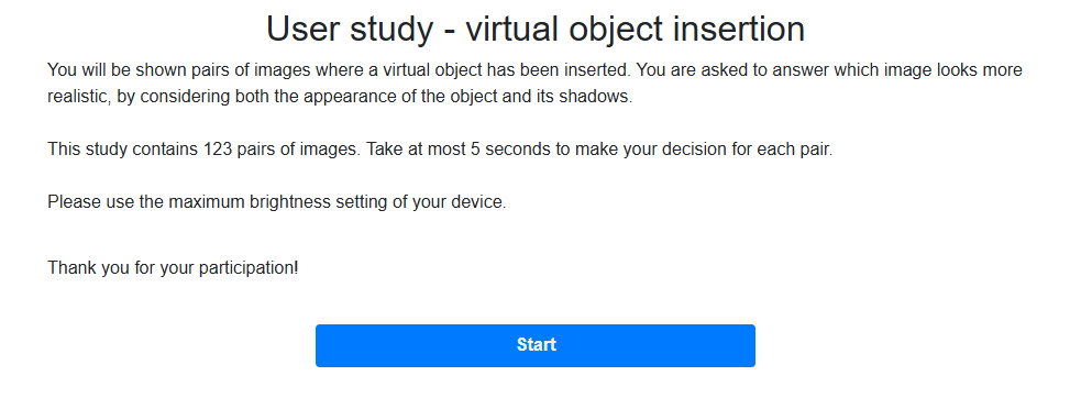
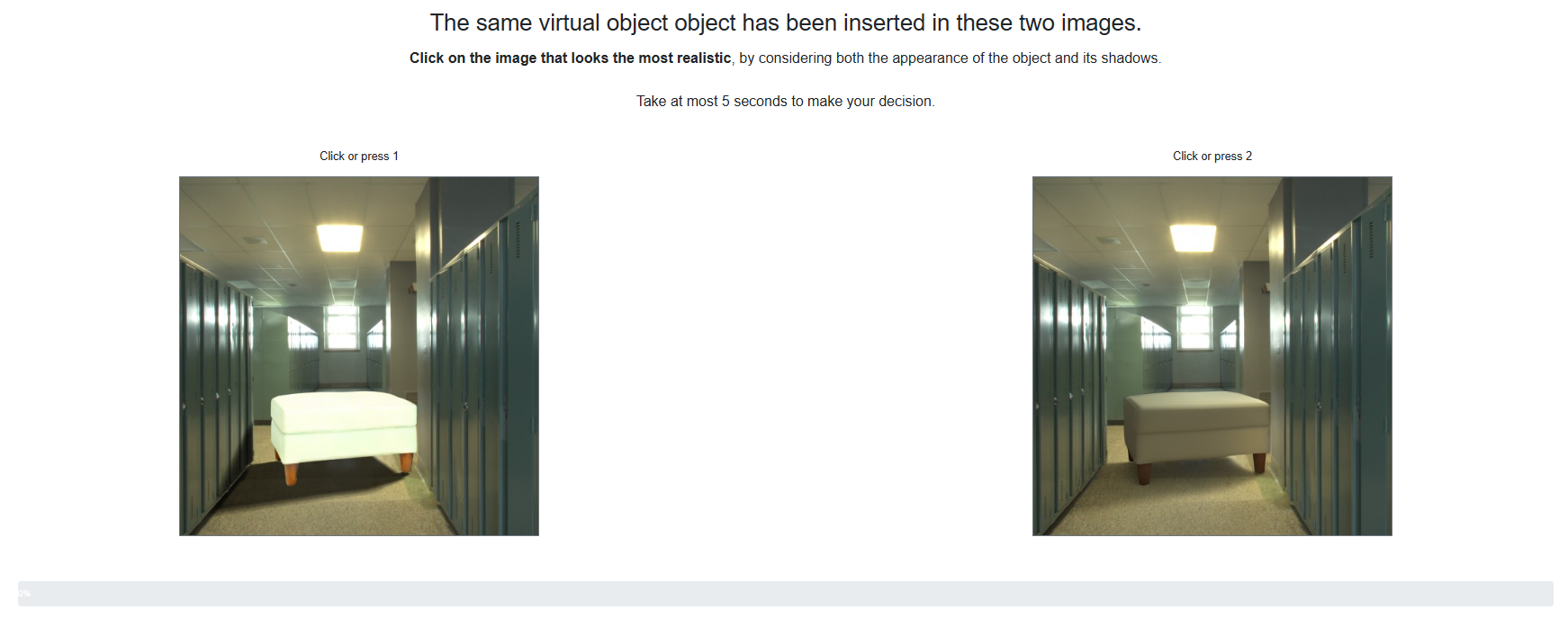
Realism study interface
Below, we show the instructions page of the overall realism user study and a question from it.
Lighting control study interface
And here, we show a video demonstration of the lighting control user study.
7. Additional results for parameters control
We show how the two main parameters of our method can be adjusted for enhanced artistic control, extending sec. 4.2 and sec. 4.3. Here, both parameters are modified separately, but they could be modified simultaneously for optimal results.
7.1. Guidance scale γ
Here, we show control over the guidance scale γ, extending fig. 6.
Increasing the guidance scale generally makes the dominant light source stronger.
Move the mouse vertically to adjust the guidance scale, and horizontally to adjust the light
azimuth
angle.
The current light azimuth angle is 0°.
The current guidance scale is γ=3.0.
7.2. Latent mask weight β
Here, we show control over the latent mask weight β, extending fig. 7.
Increasing the latent mask weight makes the dominant shadow darker.
Move the mouse vertically to adjust the latent mask weight, and horizontally to adjust the light
azimuth angle.
The current light azimuth angle is 0°.
The current latent weight is β=0.05.
8. Light source radius
We adjust the light source radius used to generate the coarse shadow fed to SpotLight.
Small radii lead to hard shadows, whereas higher radii generate more diffuse shadows.
Move the mouse vertically to adjust the light source radius, and horizontally to adjust the light
azimuth angle.
The current light azimuth angle is 0°.
The current light radius is 1 (default).
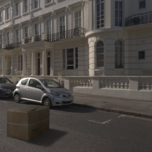
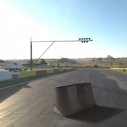
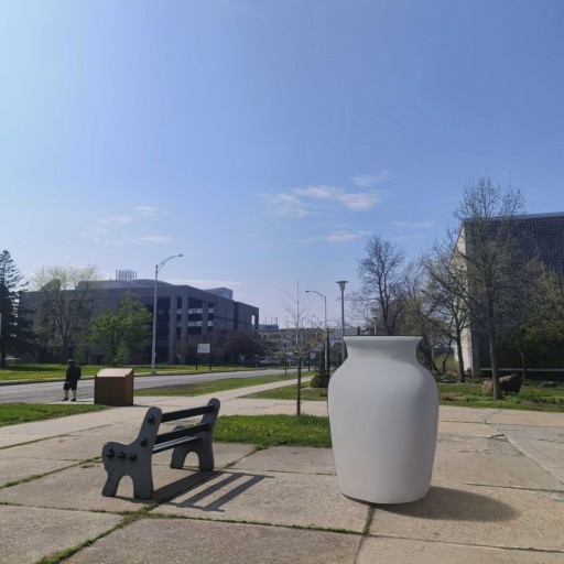
9. Outdoor scenes
Even though SpotLight relies on a diffusion renderer trained exclusively on indoor data, it can generalize to outdoor scenes well.
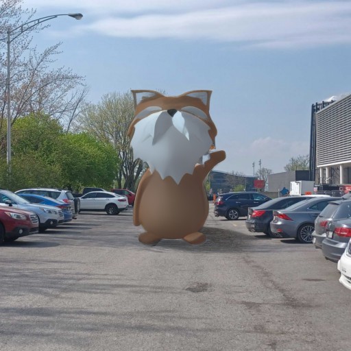
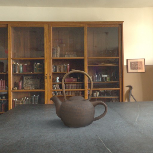
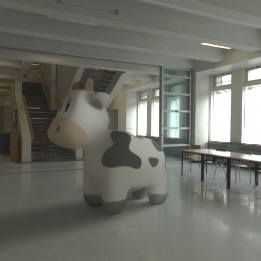
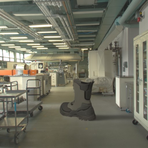
10. Diverse objects
SpotLight is not restricted to furniture and can handle many kinds of virtual objects.
11. Multiple lights
In our paper, we analyze all the methods by conditioning on a single dominant light source, which is sufficiently
realistic in most cases.
Here, we show that we can combine outputs from SpotLight at different light directions to simulate multiple light
sources.
We combine a static light direction (shadow to the right of the object), with a dynamic direction (hover over the
images to move this virtual light). We combine the two lightings
in linear space (by using the gamma of 2.2) using the following equation:
$$x_{\text{combined}}=(0.5 \times {x_{\text{light 1}}}^{2.2} + 0.5 \times {x_{\text{light
2}}}^{2.2})^{\frac{1}{2.2}}.$$
Notice how the static shadow and shading have a clear effect on the combined output.
12. Full image relighting
In our work, we use SpotLight for object relighting. We experiment with extending SpotLight for full-scene relighting using the following approach.
- We run SpotLight as-is to render the object lit with a desired shadow. We obtain the SpotLight output.
- We run the backbone (in this case ZeroComp), with the inverted shading mask, feeding it only the shading of the object and its shadow (obtained by dividing the SpotLight prediction with the albedo map) and letting the backbone shade the background. We obtain the relit background output.
- We repeat step 2 for each of the 8 light directions, and average them, giving us the average relit background.
- We find that the background relighting in step 2 and 3 poorly reconstruct the background's identity. We therefore obtain a per-pixel highlight map, by dividing the relit background prediction with the average relit background. We multiply that highlight map with the original background and obtain a more accurate output, relit background + composition.
Note about the checkpoint used for background relighting
In step 1, we use the same ZeroComp checkpoint as in all other experiments. For steps 2 and 3, in order to properly relight the background, we found that this checkpoint had limited full-scene relighting capabilities. We hypothesize that this is due to the fact that the neural renderer backbone is trained to relight only a small region of an image (circular and rectangular masks at training time). We therefore train a separate model from scratch for 270K iterations on inverted shading masks, where we take the inverse of the circular and rectangular masks for shading masking. Furthermore, we only keep the largest connected component in the mask. This leaves training examples where only a small region of the shading is known and the full background lighting needs to be inferred.